Trend Inflation, Output Gap and Trend Output Growth

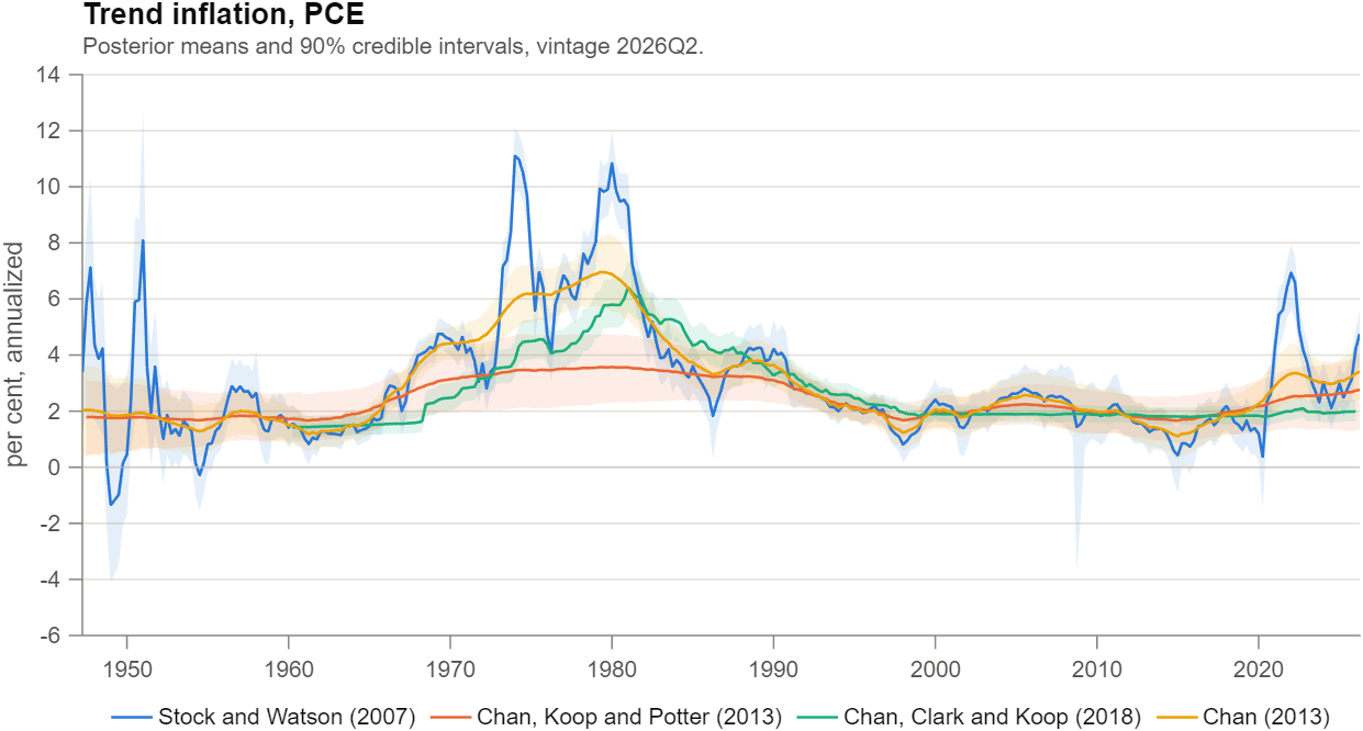
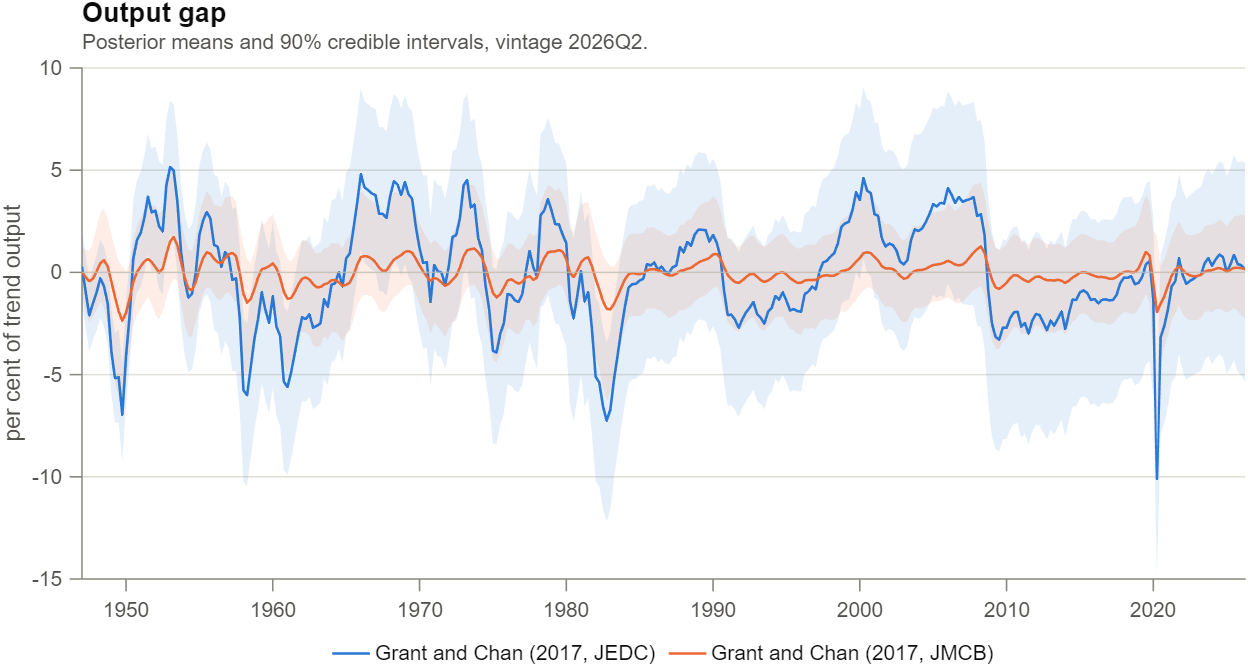
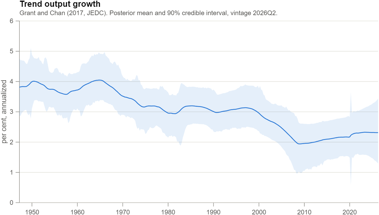
Estimates of US trend inflation, the output gap and trend output growth from six Bayesian unobserved components models, re-estimated every quarter from public data. Trend inflation is measured with the PCE price index. The figures and files on this page always show the latest release.

The models disagree, because they assume different things. Which estimate should I use? sets out what each one assumes, why their estimates differ, and which to use for which question.

Download all three series in one workbook, or as CSV files: trend inflation, output gap and trend output growth. The code, the source data behind each release, the convergence diagnostics and every past vintage are on GitHub.

Trend Inflation

• Stock and Watson (2007), the unobserved components model with stochastic volatility. Journal of Money, Credit and Banking 39(s1): 3–33.
• Chan, Koop and Potter (2013), with trend inflation bounded between 0 and 5 percent. Journal of Business and Economic Statistics 31(1): 94–106.
• Chan, Clark and Koop (2018), which adds long-run inflation expectations from the Federal Reserve Board's FRB/US model and begins in 1960. Journal of Money, Credit and Banking 50(1): 5–53.
• Chan (2013), the unobserved components model with stochastic volatility and moving average errors. Journal of Econometrics 176(2): 162–172.

What each of the four assumes, and why they differ.

@article{StockWatson2007,
  author  = {Stock, James H. and Watson, Mark W.},
  title   = {Why Has {US} Inflation Become Harder to Forecast?},
  journal = {Journal of Money, Credit and Banking},
  year    = {2007}, volume = {39}, number = {s1}, pages = {3--33}
}

@article{ChanKoopPotter2013,
  author  = {Chan, Joshua C. C. and Koop, Gary and Potter, Simon M.},
  title   = {A New Model of Trend Inflation},
  journal = {Journal of Business and Economic Statistics},
  year    = {2013}, volume = {31}, number = {1}, pages = {94--106}
}

@article{ChanClarkKoop2018,
  author  = {Chan, Joshua C. C. and Clark, Todd E. and Koop, Gary},
  title   = {A New Model of Inflation, Trend Inflation, and Long-Run Inflation Expectations},
  journal = {Journal of Money, Credit and Banking},
  year    = {2018}, volume = {50}, number = {1}, pages = {5--53}
}

@article{Chan2013,
  author  = {Chan, Joshua C. C.},
  title   = {Moving Average Stochastic Volatility Models with Application to Inflation Forecast},
  journal = {Journal of Econometrics},
  year    = {2013}, volume = {176}, number = {2}, pages = {162--172}
}

Output Gap

• Grant and Chan (2017), whose trend follows a second-order Markov process, as the Hodrick-Prescott filter implies, so that trend growth itself follows a random walk. Journal of Economic Dynamics and Control 75: 114–121.
• Grant and Chan (2017), whose trend is a random walk with a drift that takes a different value in each of the three regimes set by breaks in 1973Q1 and 2007Q1. Journal of Money, Credit and Banking 49(2–3): 525–552.

Both estimate a correlation between the trend and cycle innovations, and both allow the cycle to be serially correlated. Their estimates differ because their trends differ: what each one assumes.

@article{GrantChan2017JEDC,
  author  = {Grant, Angelia L. and Chan, Joshua C. C.},
  title   = {Reconciling Output Gaps: Unobserved Components Model and {Hodrick-Prescott} Filter},
  journal = {Journal of Economic Dynamics and Control},
  year    = {2017}, volume = {75}, pages = {114--121}
}

@article{GrantChan2017JMCB,
  author  = {Grant, Angelia L. and Chan, Joshua C. C.},
  title   = {A {Bayesian} Model Comparison for Trend-Cycle Decompositions of Output},
  journal = {Journal of Money, Credit and Banking},
  year    = {2017}, volume = {49}, number = {2-3}, pages = {525--552}
}

Trend Output Growth

From Grant and Chan (2017), Journal of Economic Dynamics and Control 75: 114–121, computed from the same draws as its output gap.

The Files

Each series is one CSV in long form: a row for every model, quarter and measure, and four columns.

mean is the posterior mean. The percentiles give the 90 percent credible interval (p05 to p95) and the 68 percent interval (p16 to p84). mcse is the Monte Carlo standard error of the posterior mean, which measures how much of the estimate is the sampler rather than the data. Trend inflation and trend output growth are in percent annualized; the output gap is in percent of trend output. trend_inflation_wide.csv holds the same posterior means with one model to a column, which is the convenient shape for a chart.

The download links above always serve the latest release. For work that has to stay reproducible, read a frozen vintage instead, which never changes once published:

https://raw.githubusercontent.com/joshuaccchan/trend-cycle-toolkit/v2026Q2.1/estimates/vintages/2026Q2/trend_inflation.csv

The tag v2026Q2.1 and the folder 2026Q2 name the vintage, and trend_inflation.csv can be replaced by output_gap.csv, trend_growth.csv or diagnostics.csv. The three examples below read that file.

import pandas as pd

url = ("https://raw.githubusercontent.com/joshuaccchan/trend-cycle-toolkit/"
       "v2026Q2.1/estimates/vintages/2026Q2/trend_inflation.csv")
df = pd.read_csv(url, parse_dates=["date"])
trend = df[(df.model == "ucsv_sw07") & (df.measure == "mean")].set_index("date")["value"]

url <- paste0("https://raw.githubusercontent.com/joshuaccchan/trend-cycle-toolkit/",
              "v2026Q2.1/estimates/vintages/2026Q2/trend_inflation.csv")
x <- read.csv(url)
x$date <- as.Date(x$date, format = "%d-%b-%Y")
trend <- x[x$model == "ucsv_sw07" & x$measure == "mean", c("date", "value")]

import delimited "https://raw.githubusercontent.com/joshuaccchan/trend-cycle-toolkit/v2026Q2.1/estimates/vintages/2026Q2/trend_inflation.csv", clear
keep if model == "ucsv_sw07" & measure == "mean"
generate day = date(date, "DMY")
generate quarter = qofd(day)
format quarter %tq
tsset quarter

Releases and Citation

New estimates are released shortly after the Bureau of Economic Analysis publishes its advance estimate of GDP, about a month after each quarter ends. Each release re-estimates the whole sample, so estimates for past quarters change as data are revised and new quarters are added. Every release is frozen and tagged on GitHub, so a vintage stays available after later releases revise it. The current tag is v2026Q2.1, which holds all six models; the earlier v2026Q2 predates the addition of Chan (2013).

Every estimate on this page is smoothed with the whole sample, so the value shown for a past quarter uses data published after it. It is not what would have been estimated at that date.

If you use the estimates, please cite the paper behind the model and the vintage you used. Work that has to stay reproducible should read the frozen vintage rather than the latest release, as The Files sets out.

@misc{Chan2026TrendCycle,
  author = {Chan, Joshua C. C.},
  title  = {trend-cycle-toolkit: {US} Trend Inflation, the Output Gap and Trend Output Growth},
  year   = {2026},
  note   = {Vintage 2026Q2, release tag v2026Q2.1},
  url    = {https://github.com/joshuaccchan/trend-cycle-toolkit}
}