How to Compare Stochastic Volatility Models by the Marginal Likelihood

Guide 4 of 4 in the series Stochastic Volatility

Based on Chan and Grant (2016)
[ Journal Version | Working Paper | Code | Full guide on GitHub ]

Chan and Eisenstat (2015)
[ Journal Version | Working Paper | Code ]

We use marginal likelihoods to choose among three models of a series: a constant variance, stochastic volatility (SV) and SV with Student-t errors (SV-t). The integrated likelihood of an SV model, with the log-volatilities integrated out, has no closed form. ssm.intlike_sv and ssm.intlike_sv_t estimate it by importance sampling. Importance sampling over the parameters then gives the marginal likelihood.

On data generated by SV, SV has the largest marginal likelihood, 0.99 above SV-t and 159.62 above the constant variance. On data generated by SV-t, SV-t has the largest, 10.33 above SV and 206.09 above the constant variance.

The steps

1. Integrate the Log-Volatilities Out
2. Draw the Parameters
3. Estimate the Marginal Likelihoods by Importance Sampling
4. Compare the Models
5. Vary the Prior of the Degrees of Freedom

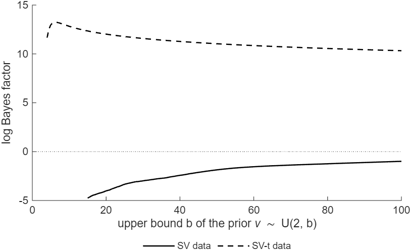
Figure 1: The log Bayes factor of SV-t against SV when ν ∼ 𝒰(2,b), against the upper bound b. Each curve starts where at least 50 posterior draws of ν lie below b. A positive value favors SV-t.

Try it

In MATLAB, from the root of a copy of statespace-toolkit, run the script that prints every number and draws every figure of the guide:

run guides/sv_compare/guide.m

In this series

Previous: How to Add Student-t Errors to a Stochastic Volatility Model