Which Parameters of a GDP Nowcasting Model Should Vary over Time?
Based on Chan, Poon and Zhu (2026)
[ Journal Version | Working Paper | Full tutorial on GitHub ]
Chan and Jeliazkov (2009)
[ Journal Version | Working Paper | Code ]
In this tutorial we nowcast US real GDP growth at the end of each month of the quarter with the mixed-data sampling (MIDAS) regressions of Chan, Poon and Zhu (2026). The predictors are monthly industrial production, the weekly National Financial Conditions Index (NFCI) and the daily spread between the 10-year and the 3-month Treasury yields. A MIDAS regression summarizes the observations of a high-frequency predictor by a weighted average, with weights from a weighting function. A coefficient multiplies the average and measures the overall impact of the predictor (Ghysels, Santa-Clara and Valkanov, 2006; Ghysels, Sinko and Valkanov, 2007). Chan, Poon and Zhu (2026) let both the coefficients and the weights vary over time. We compare five versions that switch these features on and off, and an AR(2), on the 120 quarters from 1990Q1 to 2019Q4. The nowcasts are pseudo real time: each model is re-estimated at every origin on today's revised data, with the release lags of the paper.
In this exercise, letting the coefficients vary over time improves the nowcasts, and letting the weights vary adds little. The two models whose coefficients vary, TVP-MIDAS-SV and TVP-MIDAS-SV-R1, nowcast best by every measure. Their nowcasts are nearly the same, so TVP-MIDAS-SV-R1, with fixed weights, is the simpler starting point. From the end of the second month of the quarter, their root mean squared forecast error (RMSFE) is 9 to 10 percent below the AR(2)'s. Over the same horizons, their log predictive likelihood is about 17 above that of the AR(2). Their advantage over the models with constant coefficients comes almost entirely after 2008. Letting only the weights vary, in TVP-MIDAS-SV-R2, gives the accuracy of constant parameters. Chan, Poon and Zhu (2026), with real-time data, also find the versions with only time-varying coefficients the most accurate.
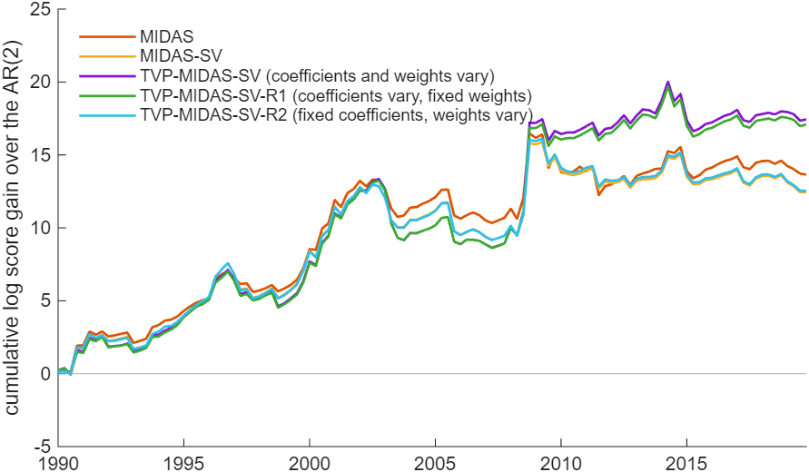
Figure 1: The cumulative difference in log predictive score of each MIDAS model against the AR(2), plotted at the target quarter. The nowcasts are made at the end of the quarter (h = 0). Every model gains on the AR(2) over the sample, most in 2008 and 2009.
Try it
In MATLAB, from the root of a copy of statespace-toolkit:
run tutorials/midas_nowcast/your_data.m: the six models on the same data with short chains, nowcasting the last two quarters at all three horizons and the quarter after the last one observed, and the exported report (about a minute)run tutorials/midas_nowcast/build.m: every number and figure in the full tutorial (about four hours with 8 CPUs)