Which Unobserved Components Model Should I Use for Inflation?
Based on Chan and Jeliazkov (2009)
[ Journal Version | Working Paper | Code | Full tutorial on GitHub ]
Chan (2013)
[ Journal Version | Working Paper | Code ]
Chan, Koop and Potter (2013)
[ Journal Version | Working Paper | Code ]
Chan, Clark and Koop (2018)
[ Journal Version | Working Paper | Code ]
In this tutorial we compare six unobserved components models of US CPI inflation by how well they forecast average inflation over the next four quarters, with an AR(4) as the benchmark. Each model splits inflation into a trend, the level at which inflation is expected to settle, and a transitory gap. Because the gap fades, the forecast of average inflation over the next year is the trend at the forecast origin plus the part of the current gap expected to persist, and averaging over four quarters removes much of the quarter-to-quarter noise in CPI inflation. In three of the six models this forecast is the trend at the origin, and in the other three the gap enters it with a weight between 0.1 and 0.3 at the end of the sample, so the forecasts depend largely on each model's estimate of the current trend, which itself is never observed.
The models use the same priors for the parameters they share, and each is re-estimated at each of 100 quarterly forecast origins from 1999Q4 to 2024Q3. Among them is UCSV, the unobserved components model with stochastic volatility of Stock and Watson (2007), in which the variances of both the trend and the gap change over time. We add UC-SVgap, which has stochastic volatility in the gap alone, to separate the two volatilities.
Every model with stochastic volatility forecasts better than the AR(4), and UC, the one model with constant variances, forecasts about as well as the AR(4). The model of Chan, Clark and Koop (2018), which also uses the SPF's 10-year inflation expectation, has the lowest root mean squared forecast error, 16 percent below the AR(4)'s. On the log predictive likelihood, it and UC-MA of Chan (2013) lead the AR(4) by 29.1 and 28.5.
Under these specifications and priors, stochastic volatility helps in the gap and not in the trend. Adding it to the gap of UC raises the log predictive likelihood by 16.3 and lowers the root mean squared forecast error from 1.95 to 1.82. Adding it to the trend as well, which gives UCSV, lowers the log predictive likelihood by 1.9 and leaves the root mean squared forecast error at 1.83. In these 100 forecasts, the root mean squared forecast error ranks the models with stochastic volatility in the same order as the average change in their forecasts from one quarter to the next.
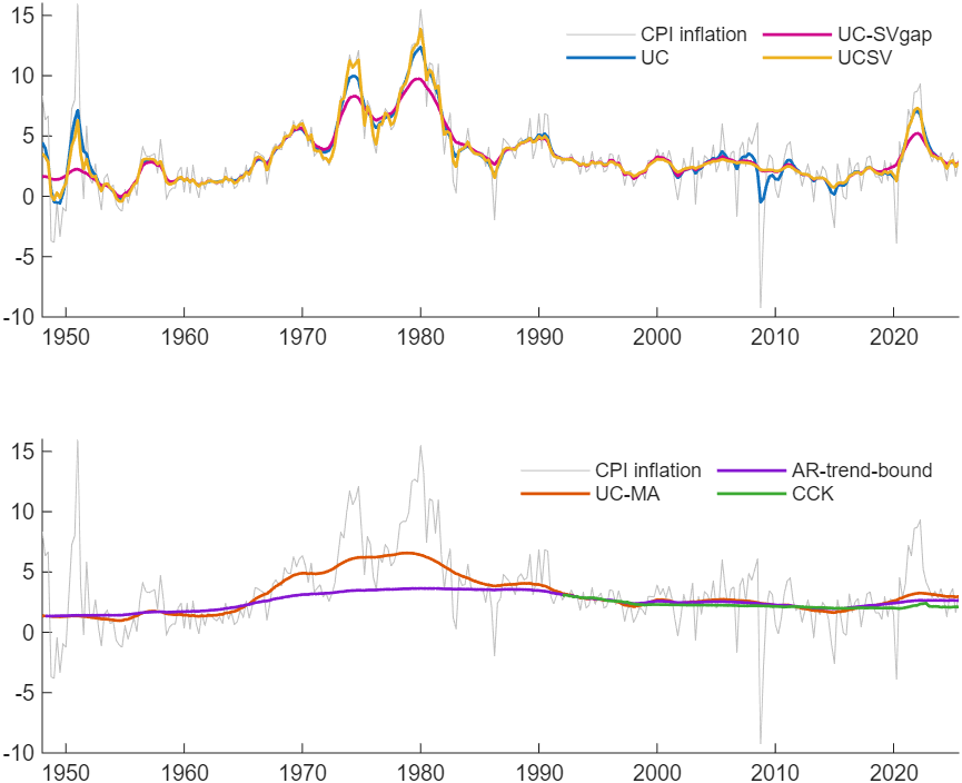
Figure 1: The posterior mean of trend inflation under each model, estimated on the whole sample, with quarterly CPI inflation in gray. Top: UC, UC-SVgap and UCSV, whose trends follow inflation closely. Bottom: UC-MA, AR-trend-bound and CCK, whose trends are smooth; the CCK trend starts in 1992Q1, when the SPF series begins.
Try it
In MATLAB, from the root of a copy of statespace-toolkit:
run tutorials/uc_specification/your_data.m: the comparison on the same data over the last six origins, with short chains, each model's forecast of the next four quarters, and the exported report (about a minute)run tutorials/uc_specification/build.m: every number and figure in the full tutorial (151 minutes)