How to Draw the VAR Coefficients under the Minnesota Prior

Guide 2 of 4 in the series Getting Started with Bayesian VARs

Based on Chan (2020)
[ Working Paper | Full guide on GitHub ]

For variables in growth rates, the Minnesota prior shrinks the coefficients of a VAR toward zero, and it shrinks those on longer lags and on the lags of other variables more strongly. In its original form the error covariance matrix is replaced by an estimate, and the coefficients then have a Gaussian posterior. One Cholesky factor of its precision matrix gives both the posterior mean and a draw. In this guide we set the prior for the VAR(2) of How to Stack the Equations of a VAR with bvar.priors.minn, compute the posterior mean and a draw with bvar.samplers.var_coef_joint, check the draws against the exact posterior, and measure how far the prior moves the estimates from least squares. Then we center the prior on a random walk.

The steps

1. Set the Prior
2. The Posterior Mean and a Draw
3. How Far the Prior Moves the Estimates

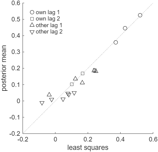
Figure 1: The posterior means of the 18 lag coefficients against their least squares estimates, by group. The dotted line marks equality.

Try it

In MATLAB, from the root of a copy of bvar-toolkit, run the script that prints every number and draws every figure of the guide:

run guides/coefficient_draw/guide.m

In this series

Previous: How to Stack the Equations of a VAR
Next: How to Estimate a VAR by Gibbs Sampling