How to Estimate a VAR by Gibbs Sampling

Guide 3 of 4 in the series Getting Started with Bayesian VARs

Based on Bayesian Macroeconometrics (Chan, forthcoming)
[ Full guide on GitHub ]

A Gibbs sampler draws the unknowns of a model in blocks, each from its distribution given the data and the current values of the other blocks, and repeats. In How to Draw the VAR Coefficients under the Minnesota Prior the error covariance matrix is replaced by an estimate, and the coefficients are drawn given it. Here Σ is unknown as well, with an inverse-Wishart prior, and the sampler alternates between two blocks: the coefficients given Σ, drawn as in that guide, and Σ given the coefficients. We run it on the VAR(2) of the earlier guides, check the chain with the diagnostics of bvar.diag, and verify the sampler under the natural conjugate prior, whose posterior is known in closed form.

The steps

1. Split the Unknowns into Blocks
2. Derive the Conditional Distributions
3. Write the Loop
4. Check the Chain

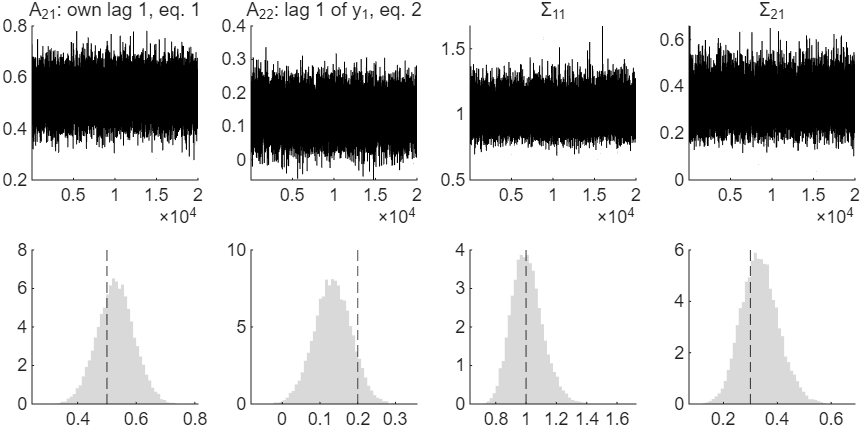
Figure 1: Top, the 20,000 draws of two coefficients and two elements of Σ kept after the burn-in, in the order the sampler makes them. Bottom, their histograms and the true values (dashed lines).

Try it

In MATLAB, from the root of a copy of bvar-toolkit, run the script that prints every number and draws every figure of the guide:

run guides/gibbs_sampler/guide.m

In this series

Previous: How to Draw the VAR Coefficients under the Minnesota Prior
Next: How to Choose the Shrinkage of a VAR by the Marginal Likelihood