How to Choose the Shrinkage of a VAR by the Marginal Likelihood

Guide 4 of 4 in the series Getting Started with Bayesian VARs

Based on Chan, Jacobi and Zhu (2020)
[ Journal Version | Working Paper | Full guide on GitHub ]

In How to Draw the VAR Coefficients under the Minnesota Prior and How to Estimate a VAR by Gibbs Sampling, the shrinkage hyperparameters of the Minnesota prior are set to commonly used values: c₁ = 0.2² for the own lags and c₂ = 0.1² for the lags of other variables. Shrinkage hyperparameters can also be chosen from the data, as the values at which the marginal likelihood, the density of the data with the parameters integrated out, is largest. Under the natural conjugate prior, a single hyperparameter controls the shrinkage of all lag coefficients, but the marginal likelihood is available in closed form. We use this prior for the data of the earlier guides, compute its log marginal likelihood, maximize it over the single hyperparameter, and see how the chosen shrinkage changes the estimates.

The steps

1. Set the Prior Variances of the Coefficients
2. Compute the Marginal Likelihood in Closed Form
3. Maximize over the Hyperparameter
4. See What the Chosen Shrinkage Does

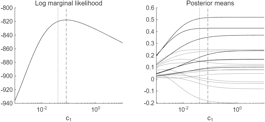
Figure 1: Left, the log marginal likelihood against c₁, on a logarithmic axis. Right, the posterior means of the 18 lag coefficients, own lags in black and lags of other variables in gray. The dashed lines mark the chosen value, c₁ = 0.081, and the dotted lines the commonly used c₁ = 0.04.

Try it

In MATLAB, from the root of a copy of bvar-toolkit, run the script that prints every number and draws every figure of the guide:

run guides/natural_conjugate_ml/guide.m

In this series

Previous: How to Estimate a VAR by Gibbs Sampling