How to Estimate a Stochastic Volatility Model by Gibbs Sampling

Guide 2 of 4 in the series Stochastic Volatility

Based on Chan and Grant (2016)
[ Journal Version | Working Paper | Code | Full guide on GitHub ]

We estimate the stochastic volatility (SV) model of How to Draw the Log-Volatilities of a Stochastic Volatility Model by Gibbs sampling, on the data of that guide. That guide holds the mean μ and the parameters μ_h, φ and σ_h² of the log-volatility at their true values. Here we estimate them along with the log-volatilities. Each iteration of the sampler draws the log-volatilities by the auxiliary mixture sampler of the first guide. It then draws three parameters from standard distributions and φ by a Metropolis-Hastings step.

The steps

1. Split the Unknowns into Blocks
2. Derive the Conditional Distributions
3. Write the Loop
4. Check the Chain

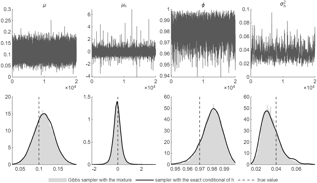
Figure 1: Top, the 20,000 draws of μ, μ_h, φ and σ_h² kept after the burn-in, in the order the sampler makes them. Bottom, their histograms over the central 99.9 percent of the draws, the posterior densities from the sampler of How We Check It, and the true values.

Try it

In MATLAB, from the root of a copy of statespace-toolkit, run the script that prints every number and draws every figure of the guide:

run guides/sv_gibbs/guide.m

In this series

Previous: How to Draw the Log-Volatilities of a Stochastic Volatility Model
Next: How to Add Student-t Errors to a Stochastic Volatility Model