How to Draw the Log-Volatilities of a Stochastic Volatility Model

Guide 1 of 4 in the series Stochastic Volatility

Based on Chan and Jeliazkov (2009)
[ Journal Version | Working Paper | Code | Full guide on GitHub ]

Chan (2017)
[ Journal Version | Working Paper | Code ]

In a stochastic volatility (SV) model, the variance of the data changes over time, and its logarithm, the log-volatility, is a state. The data depend on the state through its exponential, so the model is nonlinear, and the recipe of How to Draw the States of an Unobserved Components Model does not apply directly. The auxiliary mixture sampler of Kim, Shephard and Chib (1998) approximates the model in two steps. It takes logs of the squared data, which makes the model linear. It then approximates the distribution of the new error by a mixture of seven normal distributions. Given the mixture component of each period, the model is linear and Gaussian, and the precision sampler draws the whole path of the log-volatilities at once. In this guide the parameters are known; How to Estimate a Stochastic Volatility Model by Gibbs Sampling draws them as well.

The steps

1. Take Logs of the Squared Data
2. Approximate the Error by a Mixture of Normals
3. Alternate the Indicators and the Log-Volatilities
4. Draw from the Exact Conditional Distribution

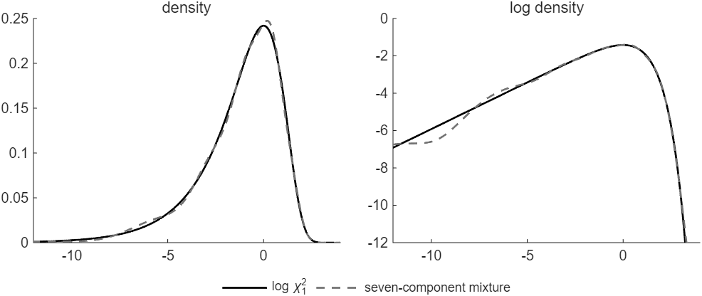
Figure 1: The density of log χ²₁ and the seven-component mixture of Kim, Shephard and Chib (1998), on a linear and on a log scale.

Try it

In MATLAB, from the root of a copy of statespace-toolkit, run the script that prints every number and draws every figure of the guide:

run guides/sv_states/guide.m

In this series

Next: How to Estimate a Stochastic Volatility Model by Gibbs Sampling