How to Draw the States of an Unobserved Components Model

Guide 1 of 3 in the series Getting Started with the Precision Sampler

Based on Chan and Jeliazkov (2009)
[ Journal Version | Working Paper | Code | Full guide on GitHub ]

In the book: Sections 9.1.1 and 9.2 of Bayesian Macroeconometrics (Chan, forthcoming)

The precision sampler draws the whole path of the states at once from their conditional distribution, 𝒩(τ̂,K^-1). It needs two inputs: the precision matrix K and the vector c with Kτ̂ = c. In this guide we draw the trend of a local level model: we stack the model's equations over time, read K and c off the log density, and call ssm.simulate_states. Then we change one equation and update K and c to match. Throughout, the parameters and the initial value of the trend are known, and we draw the trend given them and the data; How to Estimate a State Space Model by Gibbs Sampling draws the parameters as well.

The steps

1. Stack the Equations
2. Read K and c off the Log Density
3. Draw the States
4. Change One Equation

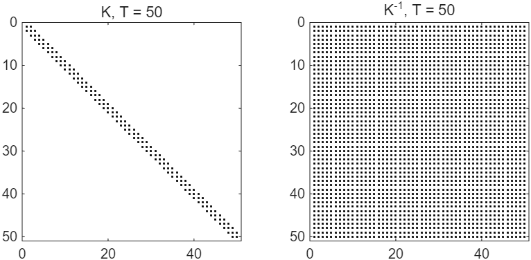
Figure 1: The nonzero entries of K and of K^-1 for the local level model with T = 50.

Try it

In MATLAB, from the root of a copy of statespace-toolkit, run the script that prints every number and draws every figure of the guide:

run guides/uc_states/guide.m

In this series

Next: How to Estimate a State Space Model by Gibbs Sampling