How to Estimate a State Space Model by Gibbs Sampling

Guide 2 of 3 in the series Getting Started with the Precision Sampler

Based on Chan and Jeliazkov (2009)
[ Journal Version | Working Paper | Code | Full guide on GitHub ]

In the book: Sections 6.3, 6.5.2 and 9.1.1 of Bayesian Macroeconometrics (Chan, forthcoming)

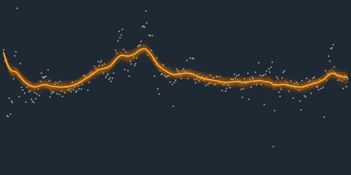
A Gibbs sampler draws the unknowns of a model in blocks, each from its distribution given the data and the current values of the other blocks, and repeats. In a state space model the states form one block, which the precision sampler draws, and the parameters form the others. In this guide we return to the local level model and the generated data of How to Draw the States of an Unobserved Components Model. That guide holds the two variances, σ² and ω², and the initial value of the trend, τ₀, at their true values; here we estimate them along with the trend. Each iteration draws the trend as in that guide and then the three parameters, each from a standard distribution.

The steps

1. Split the Unknowns into Blocks
2. Derive the Conditional Distributions
3. Write the Loop
4. Check the Chain

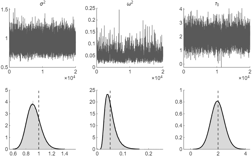
Figure 1: Top, the 20,000 draws of σ², ω² and τ₀ kept after the burn-in, in the order the sampler makes them. Bottom, their histograms, the posterior densities computed on a grid without the sampler (solid lines; see How We Check It) and the true values (dashed lines).

Try it

In MATLAB, from the root of a copy of statespace-toolkit, run the script that prints every number and draws every figure of the guide:

run guides/gibbs_sampler/guide.m

In this series

Previous: How to Draw the States of an Unobserved Components Model
Next: How to Compute the Integrated Likelihood of a State Space Model