How to Compute the Integrated Likelihood of a State Space Model

Guide 3 of 3 in the series Getting Started with the Precision Sampler

Based on Chan and Jeliazkov (2009)
[ Journal Version | Working Paper | Code | Full guide on GitHub ]

In the book: Sections 6.2.2, 6.3.2 and 9.2 of Bayesian Macroeconometrics (Chan, forthcoming)

The integrated likelihood of a state space model, also called the observed-data likelihood, is the density of the data given the parameters, with the states integrated out:

p(y | θ) = ∫p(y | α,θ) p(α | θ) dα.

Model comparison by marginal likelihood needs it, and so does any sampler that draws the parameters without the states. For a linear Gaussian model the integral has a closed form, and ssm.intlike evaluates it with the same banded precision matrix that the precision sampler uses, at a cost proportional to T. In this guide we compute it for the local level model of How to Draw the States of an Unobserved Components Model, first with the initial value of the trend known and then with it integrated out as well. We then use it to draw the two variances of How to Estimate a State Space Model by Gibbs Sampling without the states: the draws of ω², whose inefficiency factor is 27 in that guide's Gibbs sampler, become nearly independent.

The steps

1. Evaluate the Density at the Posterior Mean
2. Call ssm.intlike
3. Integrate Out the Initial Value Too
4. Draw the Variances Without the States

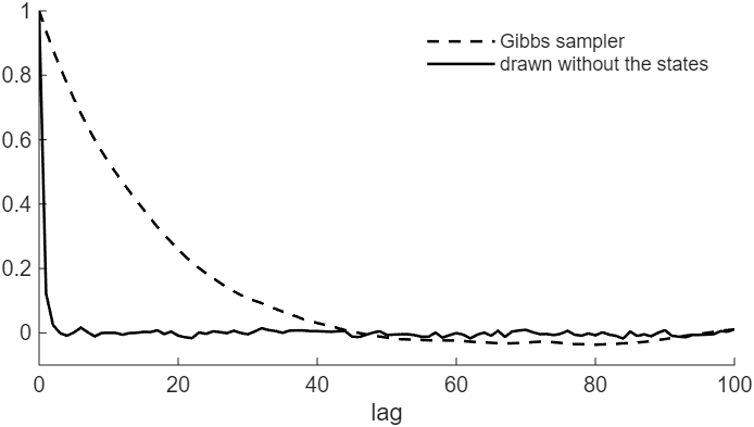
Figure 1: The autocorrelations of the 20,000 draws of ω², from the Gibbs sampler of the second guide (dashed) and from the sampler that draws the variances without the states (solid), on the same data.

Try it

In MATLAB, from the root of a copy of statespace-toolkit, run the script that prints every number and draws every figure of the guide:

run guides/integrated_likelihood/guide.m

In this series

Previous: How to Estimate a State Space Model by Gibbs Sampling