How to Forecast with a Bayesian VAR

Guide 2 of 4 in the series Forecasting with a VAR

Based on Bayesian Macroeconometrics (Chan, forthcoming)
[ Full guide on GitHub ]

The forecast of a Bayesian VAR is the predictive distribution of the future values given the data. It accounts for the shocks to come and for the uncertainty about the parameters. In this guide we estimate a VAR on 240 quarters simulated from the true model of How to Simulate Data from an Estimated VAR, draw the parameters from their posterior distribution, and simulate one future path for each draw. The point forecasts, the intervals and the probabilities of events are summaries of the paths. Because the data are simulated, we can compare these forecasts with those of the true model, made with the true parameters. We also compare them with plug-in forecasts, which fix the parameters at their posterior means.

The steps

1. Draw the Parameters from Their Posterior
2. Simulate One Path for Each Draw
3. Read the Forecasts off the Paths
4. Compare with the True Model and with Plug-in Forecasts

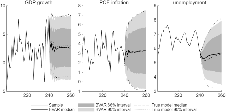
Figure 1: The forecasts of the BVAR and of the true model for the 20 quarters after the sample, with the last 40 quarters of the sample, against the quarter.

Try it

In MATLAB, from the root of a copy of bvar-toolkit, run the script that prints every number and draws every figure of the guide:

run guides/var_forecast/guide.m

In this series

Previous: How to Simulate Data from an Estimated VAR
Next: How to Evaluate Forecasts Out of Sample