Does Modeling the Volatility Improve My Forecasts?
Based on Chan (2020)
[ Journal Version | Working Paper | Code | Full tutorial on GitHub ]
Chan, Koop and Yu (2024)
[ Journal Version | Working Paper | Code ]
In this tutorial we forecast the five quarterly US series of the volatility-specification tutorial, recursively and out of sample, from three reduced-form BVARs: a homoskedastic one, one with a common volatility factor, and one with a volatility process per equation. Each is re-estimated at every forecast origin and scored two ways: by the root mean squared forecast error (RMSFE) of its point forecast, and by the log predictive likelihood of the realized value under its whole predictive density.
Over 140 forecasts from 1990 both volatility models improve on the homoskedastic benchmark by both criteria. The density gains are largest for the pandemic quarters and are not confined to them: 24 and 34 percent of the one-quarter-ahead gain and 46 and 66 percent of the four-quarter-ahead gain come from quarters before 2020. The predictive intervals show why. A homoskedastic VAR is too wide in calm years and far too narrow in a crisis.
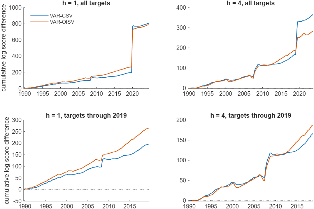
Figure 1: The running sum of the joint log predictive likelihood of each volatility model minus that of the homoskedastic VAR, against the quarter in which the forecast is made. A rising line indicates the more accurate model. The top row uses every forecast; the bottom row keeps only those whose target quarter falls before 2020, and the vertical scales differ across panels.
Try it
In MATLAB, from the root of a copy of bvar-toolkit:
run tutorials/forecasting/your_data.m: the same comparison over a short window with short chains (about a minute)run tutorials/forecasting/forecast_now.m: a forecast of the quarters after the sample, with intervals and an event probability (about a minute)run tutorials/forecasting/bench_density.m: the two ways of scoring a multi-step density, on identical draws (about a minute)run tutorials/forecasting/check_stability.m: the same quantities from chains of other seeds and four times the length (ten minutes)run tutorials/forecasting/build.m: every number and figure in the full tutorial (23 minutes)
Related tutorials
- Does the Order of the Variables Change My VAR Results?
- How Should I Choose the Shrinkage Hyperparameters of My BVAR?
- Which Stochastic Volatility Specification Should My VAR Use?