How Should I Choose the Shrinkage Hyperparameters of My BVAR?
Based on Chan (2022)
[ Journal Version | Working Paper | Code | Full tutorial on GitHub ]
In this tutorial we choose the shrinkage hyperparameters of a large Bayesian VAR by maximizing its marginal likelihood. The natural conjugate prior makes this easy, because its marginal likelihood is available in closed form, but it forces the same shrinkage on the coefficients of a variable's own lags and of other variables' lags. The asymmetric conjugate prior of Chan (2022) allows the two to differ and keeps the closed form. In the application of the working-paper version of Chan (2022), a VAR of 21 US macroeconomic and financial variables from 1959 to 2018, the marginal likelihood selects an own-lag hyperparameter of 0.41 and an other-lag hyperparameter of 0.0092, so the coefficients on other variables' lags are shrunk much more strongly (Figure 1). Imposing the same shrinkage on both lowers the maximized log marginal likelihood by 235. In recursive forecasts from 1985 to 2018, the asymmetric prior improves the one-quarter-ahead point forecasts of 20 of the 21 variables relative to the best symmetric prior, and it gives better one-quarter-ahead joint density forecasts of all 21 variables than both the symmetric prior and a subjective prior with fixed hyperparameters.
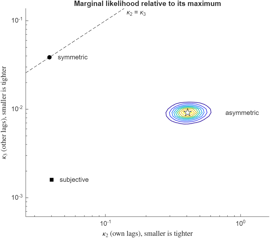
Figure 1: Marginal likelihood of the 21-variable VAR under the asymmetric conjugate prior, as a function of the own-lag hyperparameter κ2 and the other-lag hyperparameter κ3, on logarithmic axes, normalized so that its maximum equals one. Smaller values mean stronger shrinkage. The contours are at 0.1, 0.2, ..., 0.9; the star marks the maximum, the circle the best symmetric prior and the square the subjective prior, and the dashed line is the restriction κ2 = κ3.
Try it
In MATLAB, from the root of a copy of bvar-toolkit:
run tutorials/shrinkage/your_data.m: the three priors, the lag-length scan, the contour plot, forecasts and the exported report (about 15 seconds)run tutorials/shrinkage/build.m: every number and figure in the full tutorial, including the forecast comparison (about 13 minutes)
Related tutorials
- Does the Order of the Variables Change My VAR Results?
- Which Stochastic Volatility Specification Should My VAR Use?
- Does Modeling the Volatility Improve My Forecasts?